Quadratic Assignment Problem

Quadratic assignment problem (QAP) is the following problem.

Quadratic assignment problem

Let \(N\) be a positive integer. Consider \(N\) factories to be built on \(N\) candidate sites. Each factory can be built on any of the candidate sites. Every two factories have trucks traveling to and from them, and their transportation volumes are known in advance. How can we minimize the sum of the amount transported x the distance traveled?

An application could be to determine the seating chart for a meeting so that people close to each other have seats closely.

Formulation

Let \(N\) potential factory locations be denoted by land \(0\), land \(1\), … , and \(N\) factories are denoted as factories \(0\), factories \(1\), …, factories \(N-1\). Also let \(D_{i, j}\) denote the distance between land \(i\) and land \(j\), and \(F_{k, l}\) denote the transport volume between factory \(k\) and factory \(l\).

Variables

With \(N \times N\) binary variables \(q\), let \(q_{i, k}\) represent whether factory \(k\) is to be built on land \(i\).

For example, factory \(3\) will be built on land \(0\) if \(q\) has the following value.

Binary variable table

	factory 0	factory 1	factory 2	factory 3	factory 4
land 0	0	0	0	1	0
land 1	0	1	0	0	0
land 2	0	0	0	0	1
land 3	1	0	0	0	0
land 4	0	0	1	0	0

Constraints

Each row and column of the binary variable table must have exactly one variable that is 1, so we place a one-hot constraint on each row and column. Conversely, if these are satisfied, then there is only one way to determine which factory to build on which land.

Objective function

The objective function is the sum of transport volume x distance between factories. This can be expressed in the equation using \(q\) as follows.

\[ \sum_{q_{i, k} = 1, q_{j, l} = 1} D_{i, j} \ F_{k, l} = \sum_{i, j, k, l} q_{i, k} \ q_{j, l} \ D_{i, j} \ F_{k, l} \]

Formulation

The above formulation, with \(N\times N\) binary variables \(q\), can be written as follows.

\[\begin{split} \begin{align} \text{minimize} \quad &\sum_{i, j, k, l} q_{i, k} \ q_{j, l} \ D_{i, j} \ F_{k, l} \\ \text{subject to} \quad &\sum_k q_{i, k} = 1 \quad \text{for} \quad i \in \{0, 1, \ldots, N - 1\}, \\ &\sum_i q_{i, k} = 1 \quad \text{for} \quad k \in \{0, 1, \ldots, N - 1\}, \\ &q_{i, k} \in \{0, 1\} \quad \text{for} \quad i, k \in \{0, 1, \ldots, N - 1\}. \end{align} \end{split}\]

Problem setting

Before formulating with the Amplify SDK, we will create a problem. For simplicity, let the number of factories \(N=10\).

import numpy as np

N = 10

Next, we create a distance matrix \(D\) representing the distances between lands. The lands are randomly generated on the Euclidean plane. The distance matrix distance is created as a two-dimensional numpy.ndarray.

rng = np.random.default_rng()

x = rng.integers(0, 100, size=(N,))
y = rng.integers(0, 100, size=(N,))

distance = (
    (x[:, np.newaxis] - x[np.newaxis, :]) ** 2
    + (y[:, np.newaxis] - y[np.newaxis, :]) ** 2
) ** 0.5

print(distance)

[[ 0.    50.448 42.202 43.081 46.098 24.839 69.527 21.587 36.878 19.105]
 [50.448  0.    73.335 16.031 58.856 52.    21.84  45.354 31.257 65.437]
 [42.202 73.335  0.    74.545 22.672 67.007 83.815 29.275 43.417 54.406]
 [43.081 16.031 74.545  0.    64.475 38.275 37.336 45.277 37.736 54.672]
 [46.098 58.856 22.672 64.475  0.    69.34  64.938 25.239 27.659 63.325]
 [24.839 52.    67.007 38.275 69.34   0.    73.736 44.102 53.151 21.213]
 [69.527 21.84  83.815 37.336 64.938 73.736  0.    59.363 40.719 85.983]
 [21.587 45.354 29.275 45.277 25.239 44.102 59.363  0.    19.849 40.112]
 [36.878 31.257 43.417 37.736 27.659 53.151 40.719 19.849  0.    55.902]
 [19.105 65.437 54.406 54.672 63.325 21.213 85.983 40.112 55.902  0.   ]]

Also, we create a matrix \(F\) representing the amount of transport between factories, a random symmetric matrix of dimension 2, named flow.

flow = np.zeros((N, N), dtype=int)
for i in range(N):
    for j in range(i + 1, N):
        flow[i, j] = flow[j, i] = rng.integers(0, 100)

print(flow)

[[ 0 85 69 29 22 60 77 43 43  6]
 [85  0 47 13 76  4 29 53 53 64]
 [69 47  0 76 80 35 57 10 15  4]
 [29 13 76  0 97  9  0 27 32 61]
 [22 76 80 97  0 59 82 19 36 77]
 [60  4 35  9 59  0 85 35 58 56]
 [77 29 57  0 82 85  0 75 72 93]
 [43 53 10 27 19 35 75  0 25  5]
 [43 53 15 32 36 58 72 25  0 64]
 [ 6 64  4 61 77 56 93  5 64  0]]

Formulation with the Amplify SDK

In the formulation, we can use the Matrix class for efficient formulation, since a quadratic term consisting of any two binary variables can appear in the objective function.

Creating variables

To formulate using the Matrix class, VariableGenerator’s matrix() method to issue variables.

from amplify import VariableGenerator

gen = VariableGenerator()
matrix = gen.matrix("Binary", N, N)  # coefficient matrix
q = matrix.variable_array  # variables

q

\[\begin{split}\displaystyle \begin{aligned}&\left[\begin{matrix}q_{0,0}& q_{0,1}& q_{0,2}& q_{0,3}& q_{0,4}& q_{0,5}& q_{0,6}& q_{0,7}& q_{0,8}& q_{0,9}\\q_{1,0}& q_{1,1}& q_{1,2}& q_{1,3}& q_{1,4}& q_{1,5}& q_{1,6}& q_{1,7}& q_{1,8}& q_{1,9}\\q_{2,0}& q_{2,1}& q_{2,2}& q_{2,3}& q_{2,4}& q_{2,5}& q_{2,6}& q_{2,7}& q_{2,8}& q_{2,9}\\q_{3,0}& q_{3,1}& q_{3,2}& q_{3,3}& q_{3,4}& q_{3,5}& q_{3,6}& q_{3,7}& q_{3,8}& q_{3,9}\\q_{4,0}& q_{4,1}& q_{4,2}& q_{4,3}& q_{4,4}& q_{4,5}& q_{4,6}& q_{4,7}& q_{4,8}& q_{4,9}\\q_{5,0}& q_{5,1}& q_{5,2}& q_{5,3}& q_{5,4}& q_{5,5}& q_{5,6}& q_{5,7}& q_{5,8}& q_{5,9}\\q_{6,0}& q_{6,1}& q_{6,2}& q_{6,3}& q_{6,4}& q_{6,5}& q_{6,6}& q_{6,7}& q_{6,8}& q_{6,9}\\q_{7,0}& q_{7,1}& q_{7,2}& q_{7,3}& q_{7,4}& q_{7,5}& q_{7,6}& q_{7,7}& q_{7,8}& q_{7,9}\\q_{8,0}& q_{8,1}& q_{8,2}& q_{8,3}& q_{8,4}& q_{8,5}& q_{8,6}& q_{8,7}& q_{8,8}& q_{8,9}\\q_{9,0}& q_{9,1}& q_{9,2}& q_{9,3}& q_{9,4}& q_{9,5}& q_{9,6}& q_{9,7}& q_{9,8}& q_{9,9}\end{matrix}\right]\end{aligned}\end{split}\]

Creating the objective function

The matrix created above is an instance of the class Matrix, which has the following three properties.

• quadratic

• linear

• constant

quadratic is numpy.ndarray representing the coefficients of the second order terms, and its shape is (N, N, N, N) this time. quadratic[i, k, j, l] corresponds to the coefficients of q[i, k] * q[j, l]. That is, quadratic must be set to a 4-dimensional NumPy array such that quadratic[i, k, j, l] = distance[i, j] * flow[k, l]

linear and constant represent the coefficient and constant terms of the linear term, respectively, but since the objective function used in this problem contains only second order terms, we will not set them.

np.einsum("ij,kl->ikjl", distance, flow, out=matrix.quadratic)

Creating constraints

Impose a one-hot constraint on each row and column of the variable array q created in Creating variables.

from amplify import one_hot

constraints = one_hot(q, axis=1) + one_hot(q, axis=0)

Creating a combinatorial optimization model

Let’s combine the objective function and constraints to create a model.

penalty_weight = np.max(distance) * np.max(flow) * (N - 1)
model = matrix + penalty_weight * constraints

The penalty_weight is applied to the constraints to give weight to the constraints. In Amplify AE, the solver used in this example, if you do not specify appropriate weights for the constraints, the solver will search in the direction of making the objective function smaller rather than trying to satisfy the constraints, and you will not be able to find a feasible solution. See Constraints and Penalty Functions for details.

Creating a solver client

Now, we will create a solver client to perform combinatorial optimization using Amplify AE. The solver client class corresponding to Amplify AE is AmplifyAEClient class.

from amplify import AmplifyAEClient

client = AmplifyAEClient()

We also need to set the API token required to run Amplify AE.

Tip

After user registration, you can obtain a free API token that can be used for evaluation and validation purposes.

client.token = "xxxxxxxxxxxxxxxxxxxxxxxxxxxxxxxx"

We will set the solver’s timeout.

import datetime

client.parameters.time_limit_ms = datetime.timedelta(seconds=1)

Executing the solver

Finally, we will execute the solver using the created combinatorial optimization model and the solver client to find the solution to the quadratic programming problem.

from amplify import solve

result = solve(model, client)

The objective function value based on the best solution is shown below.

result.best.objective

168043.56476383813

The values of the variables in the optimal solution can be obtained in the form of a NumPy multidimensional array as follows.

q_values = q.evaluate(result.best.values)

print(q_values)

[[0. 0. 0. 0. 1. 0. 0. 0. 0. 0.]
 [1. 0. 0. 0. 0. 0. 0. 0. 0. 0.]
 [0. 0. 0. 0. 0. 0. 0. 0. 1. 0.]
 [0. 1. 0. 0. 0. 0. 0. 0. 0. 0.]
 [0. 0. 0. 0. 0. 1. 0. 0. 0. 0.]
 [0. 0. 1. 0. 0. 0. 0. 0. 0. 0.]
 [0. 0. 0. 0. 0. 0. 0. 1. 0. 0.]
 [0. 0. 0. 0. 0. 0. 0. 0. 0. 1.]
 [0. 0. 0. 0. 0. 0. 1. 0. 0. 0.]
 [0. 0. 0. 1. 0. 0. 0. 0. 0. 0.]]

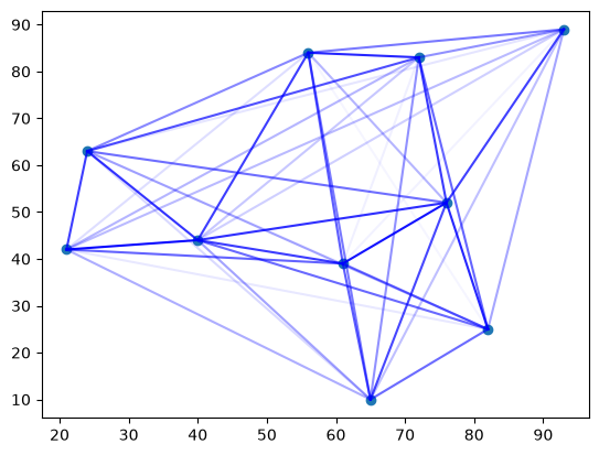
Checking the results

We will visualize the results using matplotlib.

import itertools

import matplotlib.pyplot as plt

plt.scatter(x, y)
factory_indices = (q_values @ np.arange(N)).astype(int)

for i, j in itertools.combinations(range(N), 2):
    plt.plot(
        [x[i], x[j]],
        [y[i], y[j]],
        c="b",
        alpha=flow[factory_indices[i], factory_indices[j]] / 100,
    )