Traveling Salesperson Problem
As an example of using the Amplify SDK, we will explain how to solve the traveling salesperson problem (TSP) with the Amplify SDK. The TSP is a combinatorial optimization problem that, given a set of cities, finds the shortest path that starts in one city, visits all the cities once, and returns to the first city.
Formulating the traveling salesperson problem
Let the number of cities be denoted by NUM_CITIES.
Variables
First, we will use the NUM_CITIES binary (0-1) variables to represent which of the NUM_CITIES cities is to be visited. We represent a visit to city i by setting the i-th binary variable to 1 and all other variables to 0.
For example, if the number of cities is 5 and the values of the 5 binary variables are [0, 0, 0, 0, 1, 0], this is an expression for visiting city 3, since only the variable with index 3 is 1. This method of expressing which of the n options we choose by setting one of the n binary variables to 1 is called one-hot encoding, and is often used in machine learning and other applications.
City 0 |
City 1 |
City 2 |
City 3 |
City 4 |
|---|---|---|---|---|
0 |
0 |
0 |
1 |
0 |
Since in the TSP, the salesperson visits cities one at a time and returns to the first city at the end, the number of visits to cities is NUM_CITIES + 1 times, including the first and last. So we have (NUM_CITIES + 1) * NUM_CITIES binary variables. For example, the following example represents a closed path that visits five cities in the order city 3 → city 1 → city 4 → city 0 → city 2 → city 3.
City 0 |
City 1 |
City 2 |
City 3 |
City 4 |
|---|---|---|---|---|
0 |
0 |
0 |
1 |
0 |
0 |
1 |
0 |
0 |
0 |
0 |
0 |
0 |
0 |
1 |
1 |
0 |
0 |
0 |
0 |
0 |
0 |
1 |
0 |
0 |
0 |
0 |
0 |
1 |
0 |
Constraint
In the “binary variables table” above, (NUM_CITIES + 1) * NUM_CITIES binary variables can take any value of 0 or 1, but such a path is not necessarily a close path representation. For example, having all binary variables as one yields no (closed) path. Therefore, it is necessary to impose constraints appropriately on the binary variables. Three types of constraints are required:
The first and last rows of the binary variable table must have the same value.
Each row of the binary variable table must have exactly one variable that is 1.
Each column of the binary variable table must have exactly one variable that is 1, except for the last row.
Conversely, if there is a binary variable table that satisfies the above three constraints, it represents a closed path.
Objective function
The objective of the TSP is to find the shortest route that visits all cities once and returns to the start city. Therefore, the objective function is the path length of such a route.
Suppose the distance between city i and city j is d[i, j]. The current goal is to find the path length of the closed route from the values in the binary variable table.
If the binary variable table values are known, you can find the path length of the route in the following pseudo-code. Suppose the binary variables in the ‘k’ rows and ‘i’ columns can be written as ‘q[k, i]`.
route_length = 0

for k in range(NUM_CITIES):
    for i in range(NUM_CITIES):
        for j in range(NUM_CITIES):
            route_length += (d[i, j] if q[k, i] == 1 and q[k+1, j] == 1 else 0)
However, when formulating in the Amplify SDK, we only know that each q[k, i] is a binary variable, and we do not yet know what value it will take, so we cannot make the conditional decision if q[k, i] == 1 and q[k+1, j] == 1. Only the addition and multiplication of binary variables and numbers can represent the objective function.
Now, let’s recall that the product of two binary variables q[k, i] * q[k+1, j] is 1 if q[k, i] == 1 and q[k+1, j] == 1 is true and 0 if false. Then the objective function can be implemented as follows.
route_length = 0

for k in range(NUM_CITIES):
    for i in range(NUM_CITIES):
        for j in range(NUM_CITIES):
            route_length += d[i, j] * q[k, i] * q[k+1, j]
Formulation
Writing down the above discussion in mathematical form, the formulation of the TSP in terms of binary variables (NUM_CITIES + 1) * NUM_CITIES can be written as:
However, for notational convenience, the number of cities NUM_CITIES is denoted as \(N\).
Creating problem
First, let’s create a problem. Let the number of cities be NUM_CITIES, and we will randomly select each city’s x and y coordinates from the integers 0~100. In the following, we name city 0, city 1, …, and city NUM_CITIES - 1.
This sample code sets the number of cities to 5 for simplicity.
import numpy as np
NUM_CITIES = 5
rng = np.random.default_rng()

x = rng.integers(0, 100, NUM_CITIES)
y = rng.integers(0, 100, NUM_CITIES)
Next, we will create a distance matrix representing the distances between cities. Here, the distances are Euclidean distances. The output is a NumPy array of n * n, where the elements in the i row j columns represent the distance between city i and city j, i.e. (x[i] - x[j]) ** 2 + (y[i] - y[j] ** 2) ** 0.5.
distance = (
    (x[:, np.newaxis] - x[np.newaxis, :]) ** 2
    + (y[:, np.newaxis] - y[np.newaxis, :]) ** 2
) ** 0.5

print(distance)
[[  0.     99.644  33.106  47.202  37.537]
 [ 99.644   0.     66.851 106.532  63.071]
 [ 33.106  66.851   0.     52.038  11.18 ]
 [ 47.202 106.532  52.038   0.     63.   ]
 [ 37.537  63.071  11.18   63.      0.   ]]
Formulation with the Amplify SDK
We will now formulate the problem with the Amplify SDK.
Variable generation 
First, we create the decision variables. The Amplify SDK allows you to generate variables in the form of the two-dimensional array by using VariableGenerator.
from amplify import VariableGenerator

gen = VariableGenerator()
q = gen.array("Binary", (NUM_CITIES + 1, NUM_CITIES))
The binary variables q look like the following.
q
Creating constraints 
Next, we create constraints. As described above, there are three types of constraints.
The first and last rows of the binary variable table must have the same value.
Each row of the binary variable table must have exactly one variable that is 1.
Each column of the binary variable table must have exactly one variable that is 1, except for the last row.
First constraint
Create the first constraint “the first and last rows of the binary variable table must have the same value.” is constructed here. We want to fix the last row to the same value as the first row, so we assign the first row to the last row of q. The first row of q can be written as q[0] and the last row of q as q[-1].
q[-1] = q[0]

q
We can now express the first constraint.
Attention
If you fix variables by assignment, do so before constructing the objective function or other constraints.
In subsequent constraint construction, we will not need to consider the last row of the binary variable array q, so we will create an array with the NUM_CITIES rows cut out from the top of q.
q_upper = q[:-1]

q_upper
Second constraint
We now create the second constraint, “each row of the binary variable table must have exactly one variable that is 1.” If you want to impose the constraint that exactly one of several binary variables is 1, use the one_hot() function. If you want to impose the one-hot constraint on each row of a variable array, set 1 to the axis keyword argument of the one_hot() function.
from amplify import one_hot

constraints2 = one_hot(q_upper, axis=1)

constraints2
NUM_CITIES (= 5) constraints were generated at once.
Third constraint
We then create the third constraint “each column of the binary variable table must have exactly one variable that is 1, except for the last row.” As with the second constraint, we use the one_hot() function. If you want to impose a one-hot constraint on each column of the variable array, give 0 to the axis keyword argument of the one_hot() function.
constraints3 = one_hot(q_upper, axis=0)

constraints3
Creating the objective function 
Next, we create the objective function. As mentioned above, the objective function is the path length of the route and can be written as follows.
route_length = 0

for k in range(NUM_CITIES):
    for i in range(NUM_CITIES):
        for j in range(NUM_CITIES):
            route_length += distance[i, j] * q[k, i] * q[k + 1, j]

print(route_length)
99.6443676280802 q_{0,0} q_{1,1} + 33.1058907144937 q_{0,0} q_{1,2} + 47.2016948848238 q_{0,0} q_{1,3} + 37.5366487582469 q_{0,0} q_{1,4} + 99.6443676280802 q_{0,0} q_{4,1} + 33.1058907144937 q_{0,0} q_{4,2} + 47.2016948848238 q_{0,0} q_{4,3} + 37.5366487582469 q_{0,0} q_{4,4} + 99.6443676280802 q_{0,1} q_{1,0} + 66.8505796534331 q_{0,1} q_{1,2} + 106.531685427388 q_{0,1} q_{1,3} + 63.0713881248859 q_{0,1} q_{1,4} + 99.6443676280802 q_{0,1} q_{4,0} + 66.8505796534331 q_{0,1} q_{4,2} + 106.531685427388 q_{0,1} q_{4,3} + 63.0713881248859 q_{0,1} q_{4,4} + 33.1058907144937 q_{0,2} q_{1,0} + 66.8505796534331 q_{0,2} q_{1,1} + 52.0384473250308 q_{0,2} q_{1,3} + 11.1803398874989 q_{0,2} q_{1,4} + 33.1058907144937 q_{0,2} q_{4,0} + 66.8505796534331 q_{0,2} q_{4,1} + 52.0384473250308 q_{0,2} q_{4,3} + 11.1803398874989 q_{0,2} q_{4,4} + 47.2016948848238 q_{0,3} q_{1,0} + 106.531685427388 q_{0,3} q_{1,1} + 52.0384473250308 q_{0,3} q_{1,2} + 63 q_{0,3} q_{1,4} + 47.2016948848238 q_{0,3} q_{4,0} + 106.531685427388 q_{0,3} q_{4,1} + 52.0384473250308 q_{0,3} q_{4,2} + 63 q_{0,3} q_{4,4} + 37.5366487582469 q_{0,4} q_{1,0} + 63.0713881248859 q_{0,4} q_{1,1} + 11.1803398874989 q_{0,4} q_{1,2} + 63 q_{0,4} q_{1,3} + 37.5366487582469 q_{0,4} q_{4,0} + 63.0713881248859 q_{0,4} q_{4,1} + 11.1803398874989 q_{0,4} q_{4,2} + 63 q_{0,4} q_{4,3} + 99.6443676280802 q_{1,0} q_{2,1} + 33.1058907144937 q_{1,0} q_{2,2} + 47.2016948848238 q_{1,0} q_{2,3} + 37.5366487582469 q_{1,0} q_{2,4} + 99.6443676280802 q_{1,1} q_{2,0} + 66.8505796534331 q_{1,1} q_{2,2} + 106.531685427388 q_{1,1} q_{2,3} + 63.0713881248859 q_{1,1} q_{2,4} + 33.1058907144937 q_{1,2} q_{2,0} + 66.8505796534331 q_{1,2} q_{2,1} + 52.0384473250308 q_{1,2} q_{2,3} + 11.1803398874989 q_{1,2} q_{2,4} + 47.2016948848238 q_{1,3} q_{2,0} + 106.531685427388 q_{1,3} q_{2,1} + 52.0384473250308 q_{1,3} q_{2,2} + 63 q_{1,3} q_{2,4} + 37.5366487582469 q_{1,4} q_{2,0} + 63.0713881248859 q_{1,4} q_{2,1} + 11.1803398874989 q_{1,4} q_{2,2} + 63 q_{1,4} q_{2,3} + 99.6443676280802 q_{2,0} q_{3,1} + 33.1058907144937 q_{2,0} q_{3,2} + 47.2016948848238 q_{2,0} q_{3,3} + 37.5366487582469 q_{2,0} q_{3,4} + 99.6443676280802 q_{2,1} q_{3,0} + 66.8505796534331 q_{2,1} q_{3,2} + 106.531685427388 q_{2,1} q_{3,3} + 63.0713881248859 q_{2,1} q_{3,4} + 33.1058907144937 q_{2,2} q_{3,0} + 66.8505796534331 q_{2,2} q_{3,1} + 52.0384473250308 q_{2,2} q_{3,3} + 11.1803398874989 q_{2,2} q_{3,4} + 47.2016948848238 q_{2,3} q_{3,0} + 106.531685427388 q_{2,3} q_{3,1} + 52.0384473250308 q_{2,3} q_{3,2} + 63 q_{2,3} q_{3,4} + 37.5366487582469 q_{2,4} q_{3,0} + 63.0713881248859 q_{2,4} q_{3,1} + 11.1803398874989 q_{2,4} q_{3,2} + 63 q_{2,4} q_{3,3} + 99.6443676280802 q_{3,0} q_{4,1} + 33.1058907144937 q_{3,0} q_{4,2} + 47.2016948848238 q_{3,0} q_{4,3} + 37.5366487582469 q_{3,0} q_{4,4} + 99.6443676280802 q_{3,1} q_{4,0} + 66.8505796534331 q_{3,1} q_{4,2} + 106.531685427388 q_{3,1} q_{4,3} + 63.0713881248859 q_{3,1} q_{4,4} + 33.1058907144937 q_{3,2} q_{4,0} + 66.8505796534331 q_{3,2} q_{4,1} + 52.0384473250308 q_{3,2} q_{4,3} + 11.1803398874989 q_{3,2} q_{4,4} + 47.2016948848238 q_{3,3} q_{4,0} + 106.531685427388 q_{3,3} q_{4,1} + 52.0384473250308 q_{3,3} q_{4,2} + 63 q_{3,3} q_{4,4} + 37.5366487582469 q_{3,4} q_{4,0} + 63.0713881248859 q_{3,4} q_{4,1} + 11.1803398874989 q_{3,4} q_{4,2} + 63 q_{3,4} q_{4,3}
Alternatively, the following code creates the same objective function. This code is faster because it takes full advantage of the Amplify SDK’s features and is recommended for those familiar with the NumPy library. See Speedup Formulation for details.
from amplify import Poly, einsum

q1 = q[:-1]
q2 = q[1:]
route_length: Poly = einsum("ij,ki,kj->", distance, q1, q2)  # type: ignore

print(route_length)
99.6443676280802 q_{0,0} q_{1,1} + 33.1058907144937 q_{0,0} q_{1,2} + 47.2016948848238 q_{0,0} q_{1,3} + 37.5366487582469 q_{0,0} q_{1,4} + 99.6443676280802 q_{0,0} q_{4,1} + 33.1058907144937 q_{0,0} q_{4,2} + 47.2016948848238 q_{0,0} q_{4,3} + 37.5366487582469 q_{0,0} q_{4,4} + 99.6443676280802 q_{0,1} q_{1,0} + 66.8505796534331 q_{0,1} q_{1,2} + 106.531685427388 q_{0,1} q_{1,3} + 63.0713881248859 q_{0,1} q_{1,4} + 99.6443676280802 q_{0,1} q_{4,0} + 66.8505796534331 q_{0,1} q_{4,2} + 106.531685427388 q_{0,1} q_{4,3} + 63.0713881248859 q_{0,1} q_{4,4} + 33.1058907144937 q_{0,2} q_{1,0} + 66.8505796534331 q_{0,2} q_{1,1} + 52.0384473250308 q_{0,2} q_{1,3} + 11.1803398874989 q_{0,2} q_{1,4} + 33.1058907144937 q_{0,2} q_{4,0} + 66.8505796534331 q_{0,2} q_{4,1} + 52.0384473250308 q_{0,2} q_{4,3} + 11.1803398874989 q_{0,2} q_{4,4} + 47.2016948848238 q_{0,3} q_{1,0} + 106.531685427388 q_{0,3} q_{1,1} + 52.0384473250308 q_{0,3} q_{1,2} + 63 q_{0,3} q_{1,4} + 47.2016948848238 q_{0,3} q_{4,0} + 106.531685427388 q_{0,3} q_{4,1} + 52.0384473250308 q_{0,3} q_{4,2} + 63 q_{0,3} q_{4,4} + 37.5366487582469 q_{0,4} q_{1,0} + 63.0713881248859 q_{0,4} q_{1,1} + 11.1803398874989 q_{0,4} q_{1,2} + 63 q_{0,4} q_{1,3} + 37.5366487582469 q_{0,4} q_{4,0} + 63.0713881248859 q_{0,4} q_{4,1} + 11.1803398874989 q_{0,4} q_{4,2} + 63 q_{0,4} q_{4,3} + 99.6443676280802 q_{1,0} q_{2,1} + 33.1058907144937 q_{1,0} q_{2,2} + 47.2016948848238 q_{1,0} q_{2,3} + 37.5366487582469 q_{1,0} q_{2,4} + 99.6443676280802 q_{1,1} q_{2,0} + 66.8505796534331 q_{1,1} q_{2,2} + 106.531685427388 q_{1,1} q_{2,3} + 63.0713881248859 q_{1,1} q_{2,4} + 33.1058907144937 q_{1,2} q_{2,0} + 66.8505796534331 q_{1,2} q_{2,1} + 52.0384473250308 q_{1,2} q_{2,3} + 11.1803398874989 q_{1,2} q_{2,4} + 47.2016948848238 q_{1,3} q_{2,0} + 106.531685427388 q_{1,3} q_{2,1} + 52.0384473250308 q_{1,3} q_{2,2} + 63 q_{1,3} q_{2,4} + 37.5366487582469 q_{1,4} q_{2,0} + 63.0713881248859 q_{1,4} q_{2,1} + 11.1803398874989 q_{1,4} q_{2,2} + 63 q_{1,4} q_{2,3} + 99.6443676280802 q_{2,0} q_{3,1} + 33.1058907144937 q_{2,0} q_{3,2} + 47.2016948848238 q_{2,0} q_{3,3} + 37.5366487582469 q_{2,0} q_{3,4} + 99.6443676280802 q_{2,1} q_{3,0} + 66.8505796534331 q_{2,1} q_{3,2} + 106.531685427388 q_{2,1} q_{3,3} + 63.0713881248859 q_{2,1} q_{3,4} + 33.1058907144937 q_{2,2} q_{3,0} + 66.8505796534331 q_{2,2} q_{3,1} + 52.0384473250308 q_{2,2} q_{3,3} + 11.1803398874989 q_{2,2} q_{3,4} + 47.2016948848238 q_{2,3} q_{3,0} + 106.531685427388 q_{2,3} q_{3,1} + 52.0384473250308 q_{2,3} q_{3,2} + 63 q_{2,3} q_{3,4} + 37.5366487582469 q_{2,4} q_{3,0} + 63.0713881248859 q_{2,4} q_{3,1} + 11.1803398874989 q_{2,4} q_{3,2} + 63 q_{2,4} q_{3,3} + 99.6443676280802 q_{3,0} q_{4,1} + 33.1058907144937 q_{3,0} q_{4,2} + 47.2016948848238 q_{3,0} q_{4,3} + 37.5366487582469 q_{3,0} q_{4,4} + 99.6443676280802 q_{3,1} q_{4,0} + 66.8505796534331 q_{3,1} q_{4,2} + 106.531685427388 q_{3,1} q_{4,3} + 63.0713881248859 q_{3,1} q_{4,4} + 33.1058907144937 q_{3,2} q_{4,0} + 66.8505796534331 q_{3,2} q_{4,1} + 52.0384473250308 q_{3,2} q_{4,3} + 11.1803398874989 q_{3,2} q_{4,4} + 47.2016948848238 q_{3,3} q_{4,0} + 106.531685427388 q_{3,3} q_{4,1} + 52.0384473250308 q_{3,3} q_{4,2} + 63 q_{3,3} q_{4,4} + 37.5366487582469 q_{3,4} q_{4,0} + 63.0713881248859 q_{3,4} q_{4,1} + 11.1803398874989 q_{3,4} q_{4,2} + 63 q_{3,4} q_{4,3}
Creating a combinatorial optimization model 
We now create a combinatorial optimization model by combining the objective function and constraints constructed in “creating constraints” and “creating the objective function”.
model = route_length + (constraints2 + constraints3) * np.max(distance)

print(model)
minimize:
  99.6443676280802 q_{0,0} q_{1,1} + 33.1058907144937 q_{0,0} q_{1,2} + 47.2016948848238 q_{0,0} q_{1,3} + 37.5366487582469 q_{0,0} q_{1,4} + 99.6443676280802 q_{0,0} q_{4,1} + 33.1058907144937 q_{0,0} q_{4,2} + 47.2016948848238 q_{0,0} q_{4,3} + 37.5366487582469 q_{0,0} q_{4,4} + 99.6443676280802 q_{0,1} q_{1,0} + 66.8505796534331 q_{0,1} q_{1,2} + 106.531685427388 q_{0,1} q_{1,3} + 63.0713881248859 q_{0,1} q_{1,4} + 99.6443676280802 q_{0,1} q_{4,0} + 66.8505796534331 q_{0,1} q_{4,2} + 106.531685427388 q_{0,1} q_{4,3} + 63.0713881248859 q_{0,1} q_{4,4} + 33.1058907144937 q_{0,2} q_{1,0} + 66.8505796534331 q_{0,2} q_{1,1} + 52.0384473250308 q_{0,2} q_{1,3} + 11.1803398874989 q_{0,2} q_{1,4} + 33.1058907144937 q_{0,2} q_{4,0} + 66.8505796534331 q_{0,2} q_{4,1} + 52.0384473250308 q_{0,2} q_{4,3} + 11.1803398874989 q_{0,2} q_{4,4} + 47.2016948848238 q_{0,3} q_{1,0} + 106.531685427388 q_{0,3} q_{1,1} + 52.0384473250308 q_{0,3} q_{1,2} + 63 q_{0,3} q_{1,4} + 47.2016948848238 q_{0,3} q_{4,0} + 106.531685427388 q_{0,3} q_{4,1} + 52.0384473250308 q_{0,3} q_{4,2} + 63 q_{0,3} q_{4,4} + 37.5366487582469 q_{0,4} q_{1,0} + 63.0713881248859 q_{0,4} q_{1,1} + 11.1803398874989 q_{0,4} q_{1,2} + 63 q_{0,4} q_{1,3} + 37.5366487582469 q_{0,4} q_{4,0} + 63.0713881248859 q_{0,4} q_{4,1} + 11.1803398874989 q_{0,4} q_{4,2} + 63 q_{0,4} q_{4,3} + 99.6443676280802 q_{1,0} q_{2,1} + 33.1058907144937 q_{1,0} q_{2,2} + 47.2016948848238 q_{1,0} q_{2,3} + 37.5366487582469 q_{1,0} q_{2,4} + 99.6443676280802 q_{1,1} q_{2,0} + 66.8505796534331 q_{1,1} q_{2,2} + 106.531685427388 q_{1,1} q_{2,3} + 63.0713881248859 q_{1,1} q_{2,4} + 33.1058907144937 q_{1,2} q_{2,0} + 66.8505796534331 q_{1,2} q_{2,1} + 52.0384473250308 q_{1,2} q_{2,3} + 11.1803398874989 q_{1,2} q_{2,4} + 47.2016948848238 q_{1,3} q_{2,0} + 106.531685427388 q_{1,3} q_{2,1} + 52.0384473250308 q_{1,3} q_{2,2} + 63 q_{1,3} q_{2,4} + 37.5366487582469 q_{1,4} q_{2,0} + 63.0713881248859 q_{1,4} q_{2,1} + 11.1803398874989 q_{1,4} q_{2,2} + 63 q_{1,4} q_{2,3} + 99.6443676280802 q_{2,0} q_{3,1} + 33.1058907144937 q_{2,0} q_{3,2} + 47.2016948848238 q_{2,0} q_{3,3} + 37.5366487582469 q_{2,0} q_{3,4} + 99.6443676280802 q_{2,1} q_{3,0} + 66.8505796534331 q_{2,1} q_{3,2} + 106.531685427388 q_{2,1} q_{3,3} + 63.0713881248859 q_{2,1} q_{3,4} + 33.1058907144937 q_{2,2} q_{3,0} + 66.8505796534331 q_{2,2} q_{3,1} + 52.0384473250308 q_{2,2} q_{3,3} + 11.1803398874989 q_{2,2} q_{3,4} + 47.2016948848238 q_{2,3} q_{3,0} + 106.531685427388 q_{2,3} q_{3,1} + 52.0384473250308 q_{2,3} q_{3,2} + 63 q_{2,3} q_{3,4} + 37.5366487582469 q_{2,4} q_{3,0} + 63.0713881248859 q_{2,4} q_{3,1} + 11.1803398874989 q_{2,4} q_{3,2} + 63 q_{2,4} q_{3,3} + 99.6443676280802 q_{3,0} q_{4,1} + 33.1058907144937 q_{3,0} q_{4,2} + 47.2016948848238 q_{3,0} q_{4,3} + 37.5366487582469 q_{3,0} q_{4,4} + 99.6443676280802 q_{3,1} q_{4,0} + 66.8505796534331 q_{3,1} q_{4,2} + 106.531685427388 q_{3,1} q_{4,3} + 63.0713881248859 q_{3,1} q_{4,4} + 33.1058907144937 q_{3,2} q_{4,0} + 66.8505796534331 q_{3,2} q_{4,1} + 52.0384473250308 q_{3,2} q_{4,3} + 11.1803398874989 q_{3,2} q_{4,4} + 47.2016948848238 q_{3,3} q_{4,0} + 106.531685427388 q_{3,3} q_{4,1} + 52.0384473250308 q_{3,3} q_{4,2} + 63 q_{3,3} q_{4,4} + 37.5366487582469 q_{3,4} q_{4,0} + 63.0713881248859 q_{3,4} q_{4,1} + 11.1803398874989 q_{3,4} q_{4,2} + 63 q_{3,4} q_{4,3}
subject to:
  q_{0,0} + q_{0,1} + q_{0,2} + q_{0,3} + q_{0,4} == 1 (weight: 106.53168542738823),
  q_{1,0} + q_{1,1} + q_{1,2} + q_{1,3} + q_{1,4} == 1 (weight: 106.53168542738823),
  q_{2,0} + q_{2,1} + q_{2,2} + q_{2,3} + q_{2,4} == 1 (weight: 106.53168542738823),
  q_{3,0} + q_{3,1} + q_{3,2} + q_{3,3} + q_{3,4} == 1 (weight: 106.53168542738823),
  q_{4,0} + q_{4,1} + q_{4,2} + q_{4,3} + q_{4,4} == 1 (weight: 106.53168542738823),
  q_{0,0} + q_{1,0} + q_{2,0} + q_{3,0} + q_{4,0} == 1 (weight: 106.53168542738823),
  q_{0,1} + q_{1,1} + q_{2,1} + q_{3,1} + q_{4,1} == 1 (weight: 106.53168542738823),
  q_{0,2} + q_{1,2} + q_{2,2} + q_{3,2} + q_{4,2} == 1 (weight: 106.53168542738823),
  q_{0,3} + q_{1,3} + q_{2,3} + q_{3,3} + q_{4,3} == 1 (weight: 106.53168542738823),
  q_{0,4} + q_{1,4} + q_{2,4} + q_{3,4} + q_{4,4} == 1 (weight: 106.53168542738823)
We multiply the constraints by the maximum value of the distance matrix to give weight to the constraints. In Amplify AE, the solver used in this example, unless appropriate weights are specified for the constraints, the solver will move toward reducing the objective function rather than trying to satisfy the constraints and will not be able to find a feasible solution. See Constraints and Penalty Functions for details.
Creating a solver client 
Here, we will create a solver client, specify a solver for solving, and set solver parameters. The Amplify SDK supports various solvers. Here, we will use Amplify AE. The solver client class for Amplify AE is the AmplifyAEClient class.
from amplify import AmplifyAEClient

client = AmplifyAEClient()
We will set an API token required for running Amplify AE.
Tip
Register as a user to obtain a free API token that you can use for evaluation and validation purposes.
client.token = "xxxxxxxxxxxxxxxxxxxxxxxxxxxxxxxx"
We also need to set the timeout value of the solver; the unit of the timeout value of Amplify AE is ms, but since the unit of the timeout value varies from solver to solver, the timeout value can be specified uniformly by using datetime module.
import datetime

client.parameters.time_limit_ms = datetime.timedelta(seconds=1)
This completes the solver setup.
Executing the solver 
Let’s execute the solver using the created combinatorial optimization model and the solver client to solve the traveling salesperson problem.
from amplify import solve

result = solve(model, client)
The value of the objective function, i.e., the length of the closed route, can be obtained as follows.
result.best.objective
261.09099903909055
The values of the variables in the optimal solution can be obtained in the form of a multidimensional NumPy array as follows.
q_values = q.evaluate(result.best.values)

print(q_values)
[[1. 0. 0. 0. 0.]
 [0. 0. 1. 0. 0.]
 [0. 0. 0. 0. 1.]
 [0. 1. 0. 0. 0.]
 [0. 0. 0. 1. 0.]
 [1. 0. 0. 0. 0.]]
Checking the result
This is enough for a tutorial on the Amplify SDK, but we want to visualize the result.
import matplotlib.pyplot as plt

%matplotlib inline
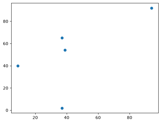
First, we visualize the locations of the cities.
plt.scatter(x, y)
plt.show()
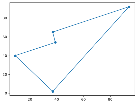
Lastly, we visualize the route. Since q_values can be considered a substitution matrix (with one row added to the end), we can sort the cities in the order they are visited on the route by multiplying the ordered vector of cities by q_values from the left.
route_x = q_values @ x  # x-coordinate of the itinerary
route_y = q_values @ y  # y-coordinate of the itinerary

plt.scatter(x, y)
plt.plot(route_x, route_y)
plt.show()