Graph Embedding#

Some QUBO and Ising solvers do not accept arbitrary second-order polynomials and are limited in the number of second-order terms that you can pass to the solver; the Amplify SDK performs an operation called graph embedding to convert the polynomial into a form that the solver can accept.

A typical example of a solver that requires graph embedding is the D-Wave machines, whose QPUs have a physical topology between the qubits that differs from machine to machine. If you view the coupling between the qubits as a graph structure, the input quadratic polynomial terms are restricted to this graph structure. This graph structure is called the physical graph, and the graph structure of the polynomial in the intermediate model constructed by the Amplify SDK is called the intermediate graph. Graph embedding is the operation to embed the intermediate graph into the physical graph.

What is graph embedding?#

Solvers that require embedding have limited types of quadratic terms they can accept as input. That is, given a set $E$ of index pairs, any quadratic terms in the input polynomial need to be expressed as:

\[ c_{ab} q_a q_b \quad (c_{ab} \in \mathbb{R}, (a, b) \in E). \]

$E$ is usually represented as a graph with the variables as nodes, where an edge connects each variable pair contained in the second-order terms that can be input.

For any polynomial, you can also look at each second-order term in the polynomial and consider the graph where an edge connects each variable pair.

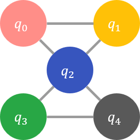
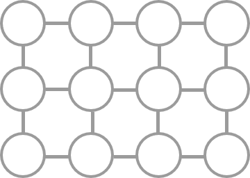
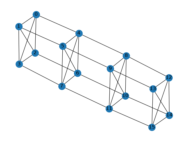
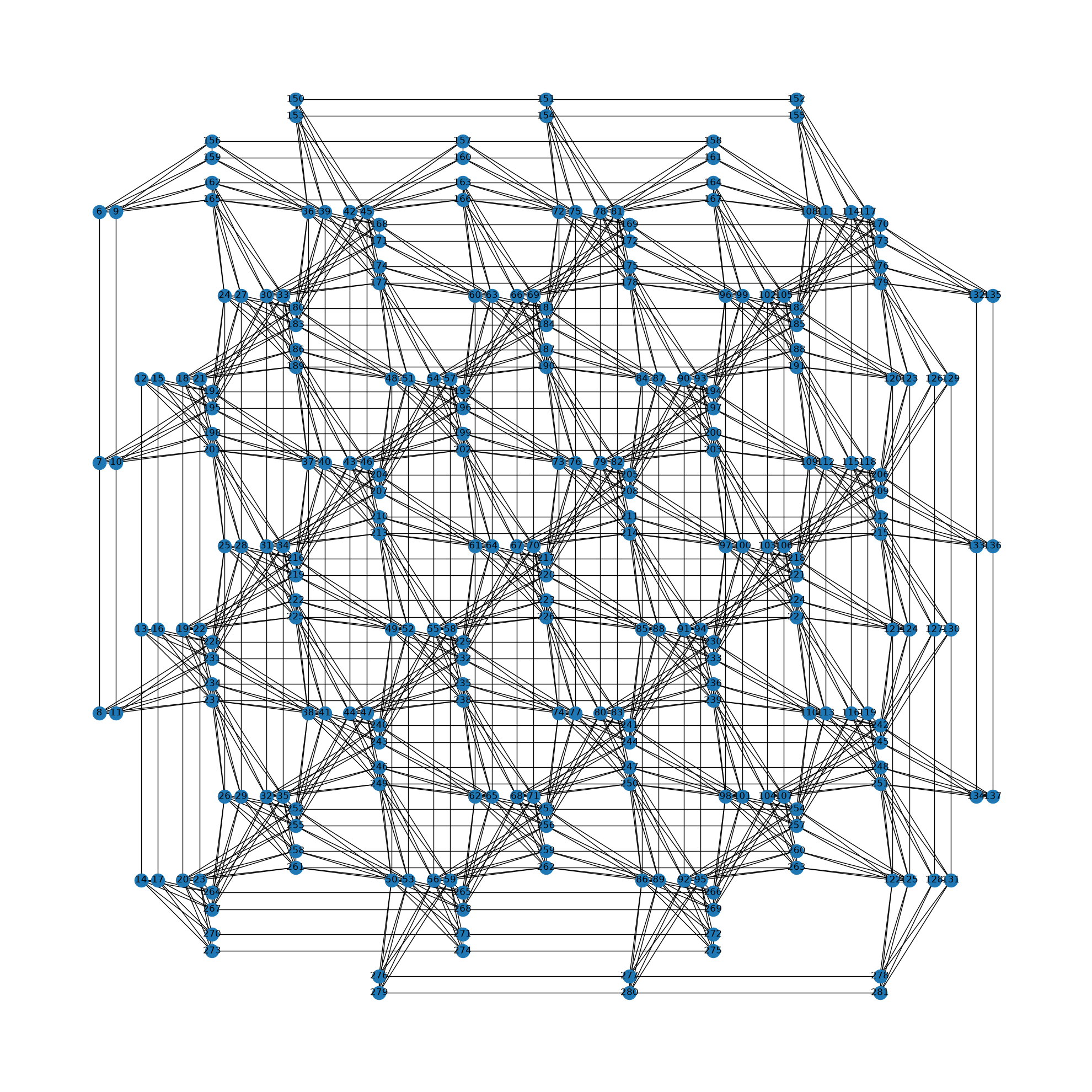
For example, suppose the objective function is $q_0 q_1 + 2 q_1 q_2 - 3 q_0 q_2 + 4 q_2 q_3 - 5 q_3 q_4 - 6 q_2 q_4$, and the graph $E$ representing the second-order terms that can be input to the solver is a $3 \times 4$ lattice graph. In that case, the graphs $P$ and $E$ of the transformed objective function are P$ and $E$, respectively, shown in the following figures.

Graph embedding is the procedure of assigning each variable in $P$ to some of the nodes in $E$ and finding the correspondence between $P$ and the nodes in $E$ such that the following conditions are satisfied.

For each variable $q_i$ on $P$, there exists one or more corresponding nodes on $E$ (one-to-many mapping is allowed).
For each node $a$ on $E$, there is at most one corresponding variable on $P$ (no duplicate assignments).
If $q_i$ and $q_j$ are neighbors on $P$, then for each of $q_i$ and $q_j$ there is a corresponding node $a$ and $b$ on $E$ that is a neighbor somewhere on $E$
For each variable $q_i$ on $P$, the subgraph of $E$ consisting of a node $a$ in $E$ corresponding to $q_i$ is connected (called a chain).

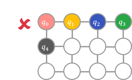
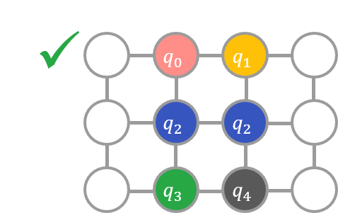
For example, if a variable is assigned to $E$ as shown in the left diagram below, the condition is not satisfied because the node to which $q_0$ is assigned is not adjacent to the node to which $q_2$ is assigned. On the other hand, if the variables are assigned as shown in the second figure below, the condition is satisfied.

_images/graph3.png — Failed graph embedding example#

_images/graph4.png — Example of successful graph embedding#

If graph embedding is successful, the objective function can be transformed into a form acceptable to the solver as follows.

Polynomial transformation by graph embedding

Second-order terms of the objective function: The second order terms $Q_{ij} q_i q_j$ of the objective function are transformed to be $\sum_{a,b} c_{ab} q_a q_b \left( Q_{ij} = \sum_{a,b} c_{ab} \right)$ and added to the new objective function. Here, $q_a$ is the variable at node $a$ on $E$ associated with $q_i$ and $q_b$ is the variable at node $b$ on $E$ associated with $q_j$, where $a$ and $b$ are adjacent.
First-order terms of the objective function: The first-order term $Q_{ii} q_i$ of the objective function is transformed to be $\sum_{a} c_{aa} q_a \left( Q_{ii} = \sum_{a} c_{aa} \right)$ and added to the new objective function, where $q_a$ is the variable at node $a$ on $E$ to which $q_i$ is assigned.
The constant term of the objective function: The constant term of the objective function is added to the new objective function as is.

Chain constraint

For a subgraph consisting of all nodes $a$ on $E$ corresponding to variables $q_i$ on $P$, add penalty functions such that variables $q_{a}$ and $q_{a'}$ on adjacent nodes satisfy the constraint $q_{a} = q_{a'}$.

The penalty function for a chain is given by

For a binary variable $q$:

\[ \sum_{a, a'} \left( q_a - q_{a'} \right)^2 \]

For an Ising variable $s$:

\[ - \frac{1}{2} \sum_{a, a'} s_a s_{a'} \]

The weight of the penalty function depends on the coefficient of $q_i$. This is called the chain strength.

The result of the solver run will be for variables on the graph $E$. Therefore, we must perform an inverse transformation of the graph embedding to determine the values of the variables on the original graph $P$. More than one variable $q_a$ in the graph $E$ corresponds to a variable $q_i$ in the graph $P$. Ideally, the values $q_a$ of all variables should be the same, but the solver may return different values in practice. Such a situation is called a broken chain, and the fraction of the chain that is broken for a polynomial on a given physical graph is called the chain break fraction. The broken chain is often determined by “majority rule” when $q_i$ is a binary variable.

Graph embedding process#

The solve() function automatically performs graph embedding after constructing the intermediate model and then runs the solver. The following is a detailed description of the graph embedding process performed by the Amplify SDK within the solve() function.

Below is an example of graph embedding for DWaveSamplerClient on a model with an objective function and constraints of $4 \times 4$ binary variables.

from amplify import DWaveSamplerClient, VariableGenerator, Model, equal_to, to_edges
import numpy as np

# Generate Variables
gen = VariableGenerator()
q = gen.array("Binary", shape=(4, 4))

# Define an objective function and a constraint
rng = np.random.default_rng()
p = (q[:-1] * q[1:] * rng.uniform(-1, 1, (3, 4))).sum()
c = equal_to(q, 1, axis=1)

# Create an input model
m = p + c

# Create a solver client
client = DWaveSamplerClient()

Polynomial to graph conversion#

First, the Amplify SDK uses the to_intermediate_model() method to obtain the intermediate model. This operation is not mandatory since the model, in this case, consists of quadratic binary variables, but it is necessary in case of variable conversion or order reduction.

im, im_mapping = m.to_intermediate_model(client.acceptable_degrees)

Next, since DWaveSamplerClient cannot handle constraints directly, the Amplify SDK computes a polynomial by adding all constraint penalties to the objective function.

im_unconstrained = im.to_unconstrained_poly()

We now have the intermediate model as a quadratic polynomial in binary variables. You can obtain the graph representation of the quadratic polynomial using the to_edges function. If a node of the graph is represented by the variable id, the function returns the edges as a list of tuples of id. The first-order term is represented as a loop.

edges = to_edges(im_unconstrained)

>>> im_unconstrained.variables
[Variable({name: q_{0,0}, id: 0, type: Binary}),
 Variable({name: q_{0,1}, id: 1, type: Binary}),
 Variable({name: q_{0,2}, id: 2, type: Binary}),
 ...
]
>>> edges
[(0, 4), (1, 5), (2, 6), (3, 7), (4, 8), (5, 9), (6, 10), ...]

Using the networkx module, you can visualize the graph.

import networkx as nx

g = nx.Graph()
g.add_edges_from(edges)
g.remove_edges_from(nx.selfloop_edges(g))
nx.draw(g, with_labels=True)

_images/cf5ee62596995c489ad2f96b1086594f70ece4674b1cac581c1f99848fbcc70c.png

Getting the physics graph#

Solver client classes that require graph embedding have a graph attribute. This attribute is an instance of the Graph class and represents the solver’s physical graph. The Graph class has the following attributes.

Attribute	Deta type	Details
`type`	`str`	Graph type
`shape`	`list`[`int`]	Graph size parameter
`nodes`	`list`[`int`]	List of nodes in the graph
`edges`	`list`[`tuple`[`int`, `int`]]	List of graph edges
`adjacency`	`list`[`list`[`int`]]	List of neighbor nodes for each node

As an example, let us obtain the graph attribute for DWaveSamplerClient.

from amplify import DWaveSamplerClient

client = DWaveSamplerClient()
client.solver = "Advantage_system4.1"
graph = client.graph

>>> graph.type
'Pegasus'
>>> graph.shape
[16]
>>> len(graph.nodes)
5627
>>> len(graph.edges)
40279

You can visualize the physical graph by drawing edges with the networkx module. On the other hand, the dwave_networkx module can be used to draw the graph in a well-formed layout according to shape. The following figure shows an example of a Pegasus graph (shape=4).

import dwave_networkx as dnx

p = dnx.pegasus_graph(4)
dnx.draw_pegasus(p, with_labels=True)

_images/a41db8da1d80ec2ed76000953b5d7217ad3a44e469cac5256f0e985fdcf8ec06.png — Pegasus graph (`shape=4`)#

Executing a graph embedding#

Call the embed() function to perform a graph embedding and get the embedding information. This function takes an instance of the polynomial Poly and Graph classes as arguments and returns a tuple consisting of the polynomial after graph embedding, the mapping of the graph embedding, and a graph converted from the argument polynomial.

from amplify import embed

# Perform graph embedding on a D-Wave graph.
emb_poly, embedding, src_graph = embed(im_unconstrained, graph)

emb_poly returns a polynomial transformed by graph embedding. embedding is a list of mappings (chains) from the id used in im_unconstrained to the id that appears in emb_poly. The index of the list is the id used in im_unconstrained.

>>> embedding
[array([ 180,  181, 2940], dtype=uint32),
 array([ 195,  196, 2955], dtype=uint32),
 array([ 150,  151, 2970], dtype=uint32),
 array([ 165,  166, 2985], dtype=uint32),
 ...]

src_graph is the graph representation of im_unconstrained. Applying the to_edges function to im_unconstrained returns the same result.

Using the dwave_networkx module, you can visualize graph embedding.

p = dnx.pegasus_graph(*graph.shape)
dnx.draw_pegasus_embedding(
    p,
    emb={i: v.tolist() for i, v in enumerate(embedding)},
    embedded_graph=g,
    show_labels=True
)

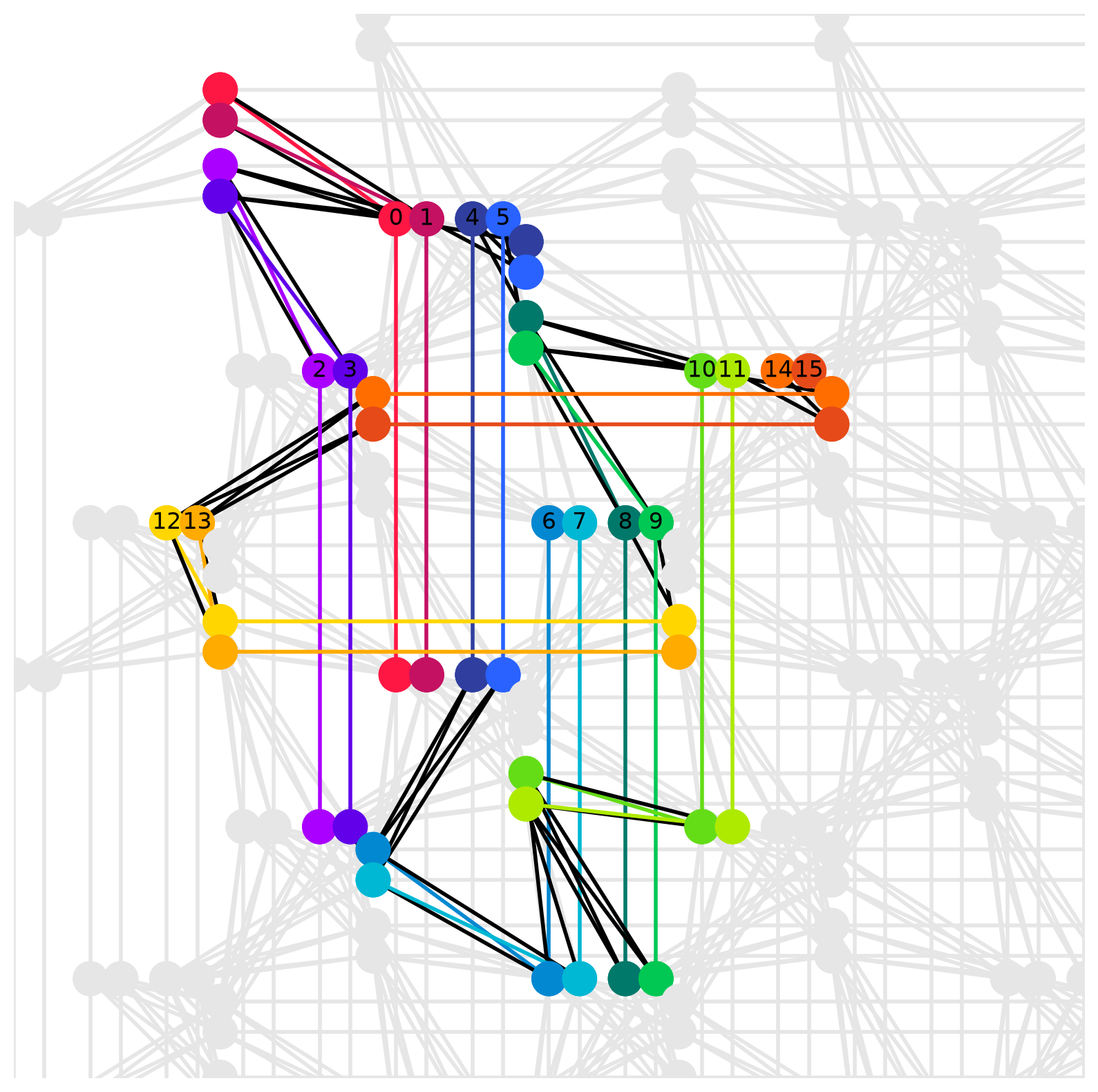
_images/c84a99cdc80ce10c75db38392bf9a91bd70b14864d5180131b4b7b08c94fec53.png — Example of graph embedding into a Pegasus graph (`shape=16`)#

In the figure above, the numbers on the nodes represent the id variable of the im_unconstrained polynomial before embedding. Multiple nodes connected by the same color represent a chain, corresponding to a single variable before embedding. Also, black lines connecting nodes of different colors represent edges on the physical graph corresponding to second-order terms in the pre-embedded polynomial im_unconstrained.

Graph embedding execution parameters#

The Amplify SDK provides the following parameters for graph embedding execution. Embedding execution parameters can be specified as keyword arguments to the solve() and embed() functions.

Parameter	Description
`embedding_timeout`	Timeout for graph embedding search
`embedding_method`	Graph embedding algorithm
`chain_strength`	Weight of the chain penalty to add to the objective function

Embedding timeout#

You can specify a timeout for embedding a graph by passing a number or a datetime.timedelta object as the embedding_timeout keyword argument to the solve() or embed() function. The default is 10 seconds.

Embedding algorithms#

The Amplify SDK provides the following embedding algorithms. To specify an embedding algorithm, use the embedding_method keyword argument of the solve() function or the embed() function.

Clique

Search for embeddings of fully connected graphs that have the same number of nodes in the graph to be embedded.

Once found, the clique embedding is cached. Caching can be used for fast searches since it depends only on the number of nodes in the target graph. However, the maximum number of nodes for a clique embedding is determined only by the physical graph, so it will always fail for graphs that inherently have more nodes than can be embedded.

Minor

Perform minor embedding with minorminer.

If the target graph is sparse, you can expect more efficient (shorter chain) embedding than Clique embedding. This algorithm may succeed for the graph size for which Clique embedding would fail.

The embedding_timeout keyword argument sets the search timeout.

Default (Default)

First, try Clique embedding, and switch to Minor if it fails.

Parallel

Perform Clique and Minor embeddings in parallel, and select the result with fewer variables in the chain.

Chain strength#

When transforming the objective function for graph embedding, a chain constraint is applied to ensure that all nodes assigned to the same input variables take the same value. The Amplify SDK automatically adds a chain constraint penalty to the post-embedding polynomial, where the initial value of the penalty weight is the square root of the second-order coefficients of the pre-embedding polynomial divided by the number of variables. You can set the relative weight of this penalty by passing the chain_strength keyword argument to the solve() or embed() function. The default is 1.0.

Important

The above initial setting for root-mean-square is based on the D-Wave implementation. The calculation method in the Amplify SDK may change in the future.

Solver execution results and graph transformations#

When a solver that requires graph embedding is specified, the Amplify SDK performs the graph embedding in the solve() function. The embedding information is stored as an instance of the GraphConversion class in the embedding attribute of the Result class returned by the solve() function.

Note

The embedding attribute returns None for solvers that do not require graph embedding.

The GraphConversion class has the following attributes.

Attribute	Data type	Details
`src_graph`	`list`[`tuple`[`int`, `int`]]	Representation of a graph of polynomial equations, adding the intermediate model’s objective function and the constraints’ penalty.
`dst_graph`	`Graph`	Solver-specific physical graph
`chains`	`list`[`numpy.ndarray`]	List of correspondences between the `id`’s of variables in the intermediate model and the `id`’s of variables in the physical graph
`poly`	`Poly`	Resulting polynomial of graph embedding for polynomials in the intermediate model
`num_variables`	`int`	Number of `poly` variables
`values_list`	`ValuesList`	Solutions returned by the solver
`chain_break_fractions`	`ChainBreakFractions`	Percentage of chain breaks in each solution returned by the solver

For example, you can obtain the graph embedding information from running the solve() function with DWaveSamplerClient on the following model.

from amplify import VariableGenerator, Model, DWaveSamplerClient, solve

gen = VariableGenerator()
q = gen.array("Binary", 3)

objective = q[0] * q[1] + 2 * q[1] * q[2] - 3 * q[0] * q[2]
model = Model(objective)

client = DWaveSamplerClient()
client.token = "xxxxxxxxxxxxxxxxxxxxxxxxxxxxxxxx"

result = solve(model, client)

With the src_graph attribute you can obtain a list of edges transformed from the polynomial with the penalty functions of the intermediate model.

>>> result.embedding.src_graph
[(0, 1), (1, 2), (0, 2)]

You can examine the id’s of the variables in the polynomial of the intermediate model as follows.

>>> im_unconstrained = result.intermediate.model.to_unconstrained_poly()
>>> print(im_unconstrained)
q_0 q_1 - 3 q_0 q_2 + 2 q_1 q_2
>>> im_unconstrained.variables
[Variable({name: q_0, id: 0, type: Binary}),
 Variable({name: q_1, id: 1, type: Binary}),
 Variable({name: q_2, id: 2, type: Binary})]

The dst_graph attribute returns an instance of the same Graph class as the solver client’s graph attribute as a physical graph.

>>> result.embedding.dst_graph.type
'Pegasus'
>>> result.embedding.dst_graph.shape
[16]

The chains attribute represents a mapping between variables in the intermediate layer and variables in the solver. chains are a list of chains, each described as a one-dimensional ndarray object. In the following example, we see that the zeroth variable in the inter layer corresponds only to the 2940-th variable .

>>> result.embedding.chains
[array([2940], dtype=uint32), array([2955], dtype=uint32), array([45], dtype=uint32)]
>>> print(result.embedding.chains[0])
[2940]

From the poly attribute, we can get the polynomial after graph embedding. This is the same polynomial that was entered into the solver.

>>> print(result.embedding.poly)
- 3 q_{45} q_{2940} + 2 q_{45} q_{2955} + q_{2940} q_{2955}

The num_variables attribute represents the number of variables in the poly attribute. You can use this as an indicator of a problem’s simplicity; in general, the smaller the value, the easier the problem is to solve.

>>> result.embedding.num_variables
3

The values_list attribute provides a list of the solution values returned by the solver. This is a list-like object whose length is equal to the number of solutions returned by the solver, and each element corresponds to a solution returned by the solver. The solutions are represented as a dictionary, and the keys are solver variables.

>>> print(result.embedding.values_list)
[{q_{45}: 1, q_{2940}: 1, q_{2955}: 0}]

The chain_break_fractions attribute indicates the percentage of chain constraints broken for each solution returned by the solver. The appropriate value generally depends on the problem and is not necessarily 0. Suppose the value is too large to obtain a good solution. In that case, performance can be improved by providing a value greater than 1.0 for the chain_strength keyword argument of the solve() function or, conversely, a value less than 1.0 if the value is too small.

>>> print(result.embedding.chain_break_fractions)
[0]

Tip

If the Result object returned by the solve() function does not contain a solution, you can retrieve all solutions returned by the solver by setting the filter_solution property of the Result object to False. See Filtering the solution for details.