Execution Time information

The Amplify SDK provides an interface to obtain information of various execution times when solving combinatorial optimization problems.

Types of available time information

The following table shows the types of execution time information that you can obtain as datetime.timedelta objects.

amplify.Result.total_time	The total time taken by amplify.solve().
amplify.Result.response_time	The time between sending the query to the solver and receiving the response.
amplify.Result.execution_time	The time the solver used to solve the problem.
amplify.Result.Solution.time	For each solution the solver returns, this is the time from the start of the solver’s search until the solver obtains the solution.

Example of obtaining execution time

An example of obtaining execution time is shown below. First, we execute the solve() function to obtain a Result object.

from amplify import VariableGenerator, one_hot, FixstarsClient, solve
from datetime import timedelta

gen = VariableGenerator()
q = gen.array("Binary", 3)

objective = q[0] * q[1] - q[2]
constraint = one_hot(q)

model = objective + constraint

client = FixstarsClient()
# client.token = "xxxxxxxxxxxxxxxxxxxxxxxxxxxxxxxx"
client.parameters.timeout = timedelta(milliseconds=1000)

result = solve(model, client)

The total_time attribute of Result represents the time from the start to the end of the solve() function. This time includes the response time of the solver, plus the processing time taken by the Amplify SDK to perform various conversions and create the query data to pass to the solver.

>>> result.total_time 
datetime.timedelta(seconds=1, microseconds=870877)

The response_time attribute of Result represents the time between sending the request to the solver in the solve() function and receiving the response.

>>> result.response_time 
datetime.timedelta(seconds=1, microseconds=865211)

The execution_time attribute of Result represents the time taken by the solver to find the solution. This time is usually the value contained in the response from the solver.

>>> result.execution_time 
datetime.timedelta(microseconds=980543)

For each solution (Solution) in the Result, the time between starting the solver search and finding the solution can be retrieved using the time attribute. This is usually the value contained in the solver response, but if the solver does not return such information, it will be the same value as the execution_time attribute.

>>> result.best.time 
datetime.timedelta(microseconds=27925)

When the solve() function is run with the dry_run option, total_time is approximately equal to the time it took the Amplify SDK to convert the model and generate the query data. Also, response_time and execution_time will be zero.

>>> dry_run_result = solve(model, client, dry_run=True)
>>> dry_run_result.total_time 
datetime.timedelta(microseconds=59)

Plotting the time obtaining the solution

For a solver configured to return multiple solutions, we will show you how to plot the time the solver obtained each solution. Such a plot allows us to see the solver’s solutions at a given time during the solver execution. You can use the convergence of the solution to determine if the run time is too short or too long.

For example, the following figure shows how Amplify Annealing Engine (AE) updates the solution objective values for a 50-city random traveling salesperson problem.

The first step is to create the model. See “Traveling Salesperson Problem” for details on the formulation.

import numpy as np
from amplify import VariableGenerator, einsum, one_hot

N = 50
x = np.random.rand(N)
y = np.random.rand(N)
d = (
    (x[:, np.newaxis] - x[np.newaxis, :]) ** 2
    + (y[:, np.newaxis] - y[np.newaxis, :]) ** 2
) ** 0.5

gen = VariableGenerator()
q = gen.array("Binary", N + 1, N)
q[-1, :] = q[0, :]

objective = einsum("ij,ki,kj->", d, q[:-1], q[1:])
constraints = one_hot(q[:-1], axis=1) + one_hot(q[:-1], axis=0)

model = objective + d.max() * constraints

Now, we set the solver client. By default, Amplify AE returns only the best solution found, so we configure it to return all solutions found during the search.

from amplify import FixstarsClient

client = FixstarsClient()
client.parameters.timeout = 1000  # Timeout is 1000 ms
client.parameters.outputs.num_outputs = 0  # Return all solutions found

Run the solver and plot the times and objective function values of all solutions obtained.

from amplify import solve
import matplotlib.pyplot as plt

# Run the solver
result = solve(model, client)

# Get time and objective function values for each solution
times = [solution.time.total_seconds() for solution in result]
objective_values = [solution.objective for solution in result]

# Plot
plt.scatter(times, objective_values)
plt.plot(times, objective_values)
plt.xlabel("elapsed time in seconds")
plt.ylabel("objective value")
plt.grid(True)

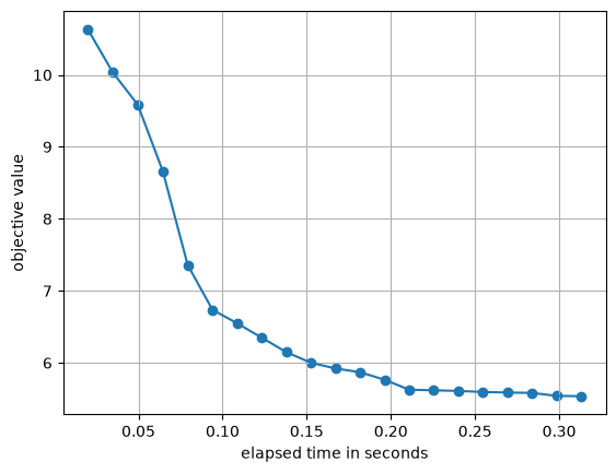
History of solutions obtained by Amplify AE for the 50-city traveling salesperson problem

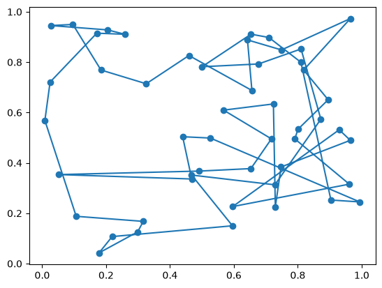
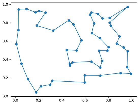
You can retrieve the initial and best solutions of the search and plot against each other as follows.

def tsp_plot(q_values, x, y):
    route_x = q_values @ x
    route_y = q_values @ y

    plt.scatter(x, y)
    plt.plot(route_x, route_y)
    plt.show()

# Plot of the initial solution
tsp_plot(q.evaluate(result[-1].values), x, y)
# Plot of the best solution
tsp_plot(q.evaluate(result[0].values), x, y)

Path (0.08 seconds) of the initial solution

Path (0.86 seconds) of the best solution