Evaluating Results

Amplify-BBOpt allows you to retrieve various results and historical data from the optimization process.

This section explains how to obtain result information based on the sample program introduced in “Optimization Example of a Test Function”.

from amplify_bbopt import Optimizer

#
# ... (definition of rastrigin_function, preprocessing, imports, etc.) ...
#

# Define the black-box function
@blackbox
def func(input_x: list[float] = x_list) -> float:  # type: ignore
    return rastrigin_function(input_x)

#
# ... (solver client definition, etc.) ...
#

# Instantiate the optimizer class
optimizer = Optimizer(blackbox=func, trainer=KMTrainer(), client=client)

# Generate initial training data (using the optimizer class method)
num_init_data = 10
optimizer.add_random_training_data(num_data=num_init_data)

# Run the optimization
optimizer.optimize(num_iterations=100)

Retrieving the best solution

Among the solutions discovered during the optimization cycles, you can retrieve the best solution — the input that gives the minimum output value of the black-box objective function — and its corresponding objective function value using Optimizer.best as shown below:

# Print the optimization results
print(f"{optimizer.best.values}")  # {'input_x': [0.12, 0.0, 0.0, -1.98, 0.0]}
print(f"{optimizer.best.objective}")  # 6.723966712641115

Tip

You can also evaluate the black-box function based on the best solution (input values) as follows:

# Evaluate the black-box function using the best solution
print(func(**optimizer.best.values))

Here, ** is Python syntax that expands the contents of a dictionary (optimizer.best.values) as keyword arguments. In the above example, this is equivalent to calling func(input_x=[0.12, 0.0, 0.0, -1.98, 0.0]).

Retrieving history information

Optimizer.history stores the complete history of all optimization cycles. It is a list of IterationResult objects, each containing various information about a single optimization cycle. Using history, you can access detailed history data related to the executed black-box optimization.

• Optimization cycle information in IterationResult

  For an explanation of “unique solutions” and “fallback solutions”, see this section.

  Attribute name	Description
  annealing_best_solution	The best solution obtained directly from annealing in each cycle (not necessarily unique solution)
  annealing_new_solution	The unique solution obtained from annealing in each cycle (None if no unique solution was found in that cycle)
  fallback_solution	The fallback solution (None if no fallback process occurred in that cycle)
  timing	Timing information (Timing class)
  amplify_result	amplify.Result object obtained from annealing in each cycle
  surrogate_model_info	Information on the surrogate model (SurrogateModelInfo class)

• Execution time information in Timing

  This records the processing time for each step of the optimization cycle.

  Attribute name	Description
  training	Execution time (in seconds) for Step 1 (train_surrogate())
  minimization	Execution time (in seconds) for Step 2 (minimize_surrogate())
  find_unique_solution	Execution time (in seconds) for Step 2a (find_unique_solution())
  fallback	Execution time (in seconds) for Step 2b (fallback_solution())
  update_dataset	Execution time (in seconds) for Step 3
  update_history	Execution time (in seconds) for Step 4

• Model information in SurrogateModelInfo

  Attribute name	Description
  corrcoef	Pearson correlation coefficient between the predicted values from the surrogate model function constructed in Step 1 (train_surrogate()) and the true values of the black-box function (details). The target samples are defined based on the lower percentile.

Example: Plotting optimization history

You can visualize various aspects of the optimization process using the information obtained from the history data.

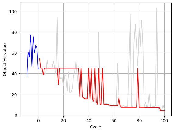
Evolution of the black-box objective values

You can plot the evaluation values of the black-box function in each optimization cycle as follows:

# Number of initial training data samples
num_initial_data = 10

# Objective values from the initial training data
objectives_init = optimizer.training_data.y[:num_initial_data]

# History of the best solutions obtained directly from annealing
objectives_annealing_best = [
    float(h.annealing_best_solution.objective) for h in optimizer.history
]

# History of the best solutions including fallback solutions
objectives_all = [
    float(h.annealing_new_solution.objective)
    if h.fallback_solution is None
    else float(h.fallback_solution.objective)
    for h in optimizer.history
]

plt.plot(range(-num_initial_data + 1, 1), objectives_init, "blue")
plt.plot(range(1, len(objectives_all) + 1), objectives_all, "lightgrey")
plt.plot(range(1, len(objectives_annealing_best) + 1), objectives_annealing_best, "-r")

plt.xlabel("Cycle")
plt.ylabel("Objective value")

plt.grid(True)

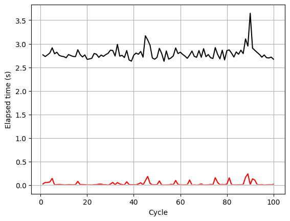
Transition of cycle execution times

You can also plot various timing information for each optimization cycle. In the following example, the total elapsed time per cycle, the time spent on annealing, and the time spent on fallback processing are shown.

cycles = range(1, len(optimizer.history) + 1)

# Total elapsed time per cycle
elapsed_total = [sum(h.timing) for h in optimizer.history]

# Time spent on annealing in each cycle
elapsed_annealing = [h.timing.minimization for h in optimizer.history]

# Time spent on fallback processing in each cycle
elapsed_fallback = [h.timing.fallback for h in optimizer.history]

plt.plot(cycles, elapsed_total, "-k")
plt.plot(cycles, elapsed_annealing, "-r")
plt.plot(cycles, elapsed_fallback, "lightgrey")

plt.xlabel("Cycle")
plt.ylabel("Elapsed time (s)")

plt.grid(True)

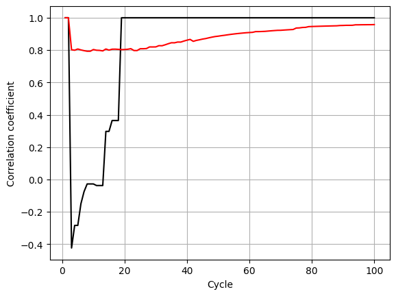
Transition of model information

You can also visualize the performance of the surrogate model function (for example, the correlation coefficient) across optimization cycles as follows:

cycles = range(1, len(optimizer.history) + 1)

# Correlation coefficient for the bottom 25% of samples (based on objective values)
tail_correlations = [
    h.surrogate_model_info.corrcoef[25] for h in optimizer.history
]

# Correlation coefficient for all samples
all_correlations = [
    h.surrogate_model_info.corrcoef[100] for h in optimizer.history
]

plt.plot(cycles, tail_correlations, "-k")
plt.plot(cycles, all_correlations, "-r")

plt.xlabel("Cycle")
plt.ylabel("Correlation coefficient")

plt.grid(True)

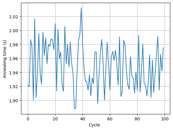
Transition of annealing information

You can also retrieve the raw results of Ising machine execution for each optimization cycle through the amplify.Result objects. Various annealing-related metrics stored in each amplify.Result (for example, the annealing execution time on the Ising machine) can be plotted as follows:

annealing_times = [
    h.amplify_result.client_result.execution_time.annealing_time.total_seconds()
    for h in optimizer.history
]

plt.plot(range(len(optimizer.history)), annealing_times)
plt.xlabel("Cycle")
plt.ylabel("Annealing time (s)")
plt.grid(True)