Maximizing Production Efficiency in a Chemical Plant

In this section, we implement a black-box optimization example — originally introduced in the Amplify SDK demos and tutorials — using Amplify-BBOpt.

The sample code we consider here is shown below. For detailed explanations of the simulator and problem setup, please refer to the following demo tutorial page:

Black-Box Optimization of Operating Condition in a Chemical Reactor In this tutorial, the goal is to optimize the operating condition of a plant reactor to maximize production. The chemical reaction and transport phenomena of reactants and products in the reactor are predicted by numerical simulations using the finite difference method. Based on the predicted results, optimization is performed to maximize the amount of material production in the reactor.

Implementation of the Reactor Simulation

Below is the implementation of the Reactor simulation class based on the finite difference method (FDM). This implementation is essentially identical to that used in the demo mentioned above.

Hide code cell source

import time

import matplotlib.pyplot as plt
import numpy as np

# A class to solve the transport equations (partial differential equations) for the concentration of a given reactive substance (A->B) by finite difference methods.


class Reactor:
    def __init__(self, nfolds=5, alpha=1.0, dt_prod=1e-3, rr=1e4):
        self.nfolds = nfolds  # Parameters that determine the spatial resolution of the simulation domain
        self.alpha = alpha  # Molecular diffusion coefficient
        self.dt_prod = dt_prod  # Predetermined production time
        self.rr = rr  # Coefficients related to the reaction rate

    # Function to compute the second-order derivative of the distribution f by second-order central differencing (assuming periodic boundary conditions)

    def __dfdx2(self, f, dfdx2):
        dfdx2[0] = (f[1] - 2 * f[0] + f[self.nx - 1]) / self.dx / self.dx
        dfdx2[self.nx - 1] = (
            (f[0] - 2 * f[self.nx - 1] + f[self.nx - 2]) / self.dx / self.dx
        )
        dfdx2[1 : self.nx - 1] = (
            np.array([
                f[i + 1] - 2 * f[i] + f[i - 1] for i in range(1, self.nx - 1)
            ])
            / self.dx
            / self.dx
        )
        return dfdx2

    # Determine the initial conditions

    def __init_field(self, x):
        self.nx = self.nfolds * len(
            x
        )  # Number of mesh points used in the spatial discretization
        self.dx = 1.0 / (self.nx - 1)  # Mesh point spacing
        self.concn_A = np.zeros(self.nx)  # Concentration distribution of A
        self.concn_B = np.zeros(self.nx)  # Concentration distribution of B
        self.x_cord = np.array([
            i / self.nx - 0.5 for i in range(self.nx)
        ])  # Coordinate of discrete points
        self.concn_A = np.array([
            float(x[i]) for i in range(len(x)) for j in range(self.nfolds)
        ])  # Generate the initial field for A

    # Function to evolve the transport equation in time by dt_prod physical time according to the initial distribution init_A of A and return the total amount of B produced

    def integrate(self, init_A, fig=False):
        self.__init_field(init_A)
        start = time.perf_counter()
        omega = np.zeros(self.nx)
        dfdx2 = np.zeros(self.nx)
        dt = (
            0.25 * self.dx * self.dx / self.alpha
        )  # Time step width in Eulerian method
        lts = int(self.dt_prod / dt)
        if fig:  # Plot of reaction progress
            fig = plt.figure(figsize=(6, 4))
            plt.tick_params(labelsize=16)
            plt.xlabel("x", fontsize=16)
            plt.ylabel("Concentration", fontsize=18)
            plt.plot(
                self.x_cord,
                self.concn_A,
                linestyle="-",
                linewidth=1,
                color=[0.6, 0.6, 0.6],
                label="$C_{A,0}$",
            )
        self.iter = 0
        while self.iter * dt < self.dt_prod:
            if fig and any([
                self.iter == i
                for i in [0, int(0.1 * lts), int(0.2 * lts), int(0.4 * lts)]
            ]):  # Plot of reaction progress
                plt.plot(
                    self.x_cord,
                    self.concn_B,
                    linestyle="-",
                    linewidth=2,
                    color="r",
                )
            omega = (
                self.rr
                * np.exp(-self.concn_B)
                * self.concn_A
                * (1.0 - self.concn_A)
            )  # Reaction rate
            self.concn_A = (
                self.concn_A
                + (self.alpha * self.__dfdx2(self.concn_A, dfdx2) - omega) * dt
            )  # Time advancement for the concentration of A
            self.concn_B = (
                self.concn_B
                + (self.alpha * self.__dfdx2(self.concn_B, dfdx2) + omega) * dt
            )  # Time advancement for the concentration of B
            self.iter += 1
        if fig:  # Plot of reaction progress
            plt.plot(
                self.x_cord,
                self.concn_B,
                linestyle="-",
                linewidth=4,
                color="r",
                label="$C_B$",
            )
            plt.legend(fontsize=16)
        self.cpu_time = (
            time.perf_counter() - start
        )  # Measure the computation time
        return (
            np.sum(self.concn_B) * self.dx
        )  # Simplified spatial integration of the concentration of B

Implementing the black-box function

Here, we implement the black-box function using the reactor simulator class Reactor together with the Amplify-BBOpt @blackbox decorator.

from logging import getLogger
from typing import Annotated

from amplify_bbopt import AMPLIFY_BBOPT_LOGGER_NAME, BinaryVariable, blackbox

logger = getLogger(AMPLIFY_BBOPT_LOGGER_NAME)

input_q = [BinaryVariable() for _ in range(100)]  # List of binary variables


# Objective function (returns the negative of the total amount of product B)
@blackbox
def my_obj_func(init_a: Annotated[list[int], input_q]) -> float:
    my_reactor = Reactor()
    minus_total = -my_reactor.integrate(init_a, fig=False)
    logger.info(f"{minus_total=:.2e}, {my_reactor.cpu_time=:.1e}s")
    return minus_total

Running the optimization

In this example, we use a Factorization Machine (FM) as the surrogate model via FMTrainer and instantiate the optimizer as FMQA. For other surrogate models, see the Model Trainer section of the documentation.

After adding the initial training data, we run the optimization cycles.

from datetime import timedelta

from amplify import FixstarsClient
from amplify_bbopt import FMTrainer, Optimizer

client = FixstarsClient()
client.parameters.timeout = timedelta(milliseconds=2000)
# client.token = "xxxxxxxxxxxxxxxxxxxxxxxxxxxxxxxx"  # Enter your Amplify AE access token when using a local environment

optimizer = Optimizer(my_obj_func, FMTrainer(), client)

num_init_data = 10  # Number of initial training samples
optimizer.add_random_training_data(num_init_data)

optimizer.optimize(10)

Hide code cell output

[2025-07-23 14:51:50] [amplify_bbopt] [INFO] Random data sample: 1/10
[2025-07-23 14:51:51] [amplify_bbopt] [INFO] minus_total=-5.55e-01, my_reactor.cpu_time=4.3e-01s
[2025-07-23 14:51:51] [amplify_bbopt] [INFO] Random data sample: 2/10
[2025-07-23 14:51:51] [amplify_bbopt] [INFO] minus_total=-5.48e-01, my_reactor.cpu_time=4.1e-01s
[2025-07-23 14:51:51] [amplify_bbopt] [INFO] Random data sample: 3/10
[2025-07-23 14:51:52] [amplify_bbopt] [INFO] minus_total=-5.19e-01, my_reactor.cpu_time=4.8e-01s
[2025-07-23 14:51:52] [amplify_bbopt] [INFO] Random data sample: 4/10
[2025-07-23 14:51:52] [amplify_bbopt] [INFO] minus_total=-5.74e-01, my_reactor.cpu_time=4.6e-01s
[2025-07-23 14:51:52] [amplify_bbopt] [INFO] Random data sample: 5/10
[2025-07-23 14:51:53] [amplify_bbopt] [INFO] minus_total=-5.38e-01, my_reactor.cpu_time=4.5e-01s
[2025-07-23 14:51:53] [amplify_bbopt] [INFO] Random data sample: 6/10
[2025-07-23 14:51:53] [amplify_bbopt] [INFO] minus_total=-4.69e-01, my_reactor.cpu_time=4.3e-01s
[2025-07-23 14:51:53] [amplify_bbopt] [INFO] Random data sample: 7/10
[2025-07-23 14:51:53] [amplify_bbopt] [INFO] minus_total=-5.58e-01, my_reactor.cpu_time=4.0e-01s
[2025-07-23 14:51:54] [amplify_bbopt] [INFO] Random data sample: 8/10
[2025-07-23 14:51:54] [amplify_bbopt] [INFO] minus_total=-4.88e-01, my_reactor.cpu_time=4.0e-01s
[2025-07-23 14:51:54] [amplify_bbopt] [INFO] Random data sample: 9/10
[2025-07-23 14:51:54] [amplify_bbopt] [INFO] minus_total=-5.44e-01, my_reactor.cpu_time=4.3e-01s
[2025-07-23 14:51:54] [amplify_bbopt] [INFO] Random data sample: 10/10
[2025-07-23 14:51:55] [amplify_bbopt] [INFO] minus_total=-5.47e-01, my_reactor.cpu_time=4.3e-01s
[2025-07-23 14:51:55] [amplify_bbopt] [INFO] === Iteration: 1/10 ===
[2025-07-23 14:52:06] [amplify_bbopt] [INFO] model corrcoefs: <=10%: nan, <=25%: 0.971, <=50%: 0.464, all: -0.366
[2025-07-23 14:52:09] [amplify_bbopt] [INFO] minus_total=-4.09e-01, my_reactor.cpu_time=4.0e-01s
[2025-07-23 14:52:09] [amplify_bbopt] [INFO]    objective: -4.094e-01
[2025-07-23 14:52:09] [amplify_bbopt] [INFO] current best: -5.742e-01
[2025-07-23 14:52:09] [amplify_bbopt] [INFO] === Iteration: 2/10 ===
[2025-07-23 14:52:16] [amplify_bbopt] [INFO] model corrcoefs: <=10%: 1.000, <=25%: 0.994, <=50%: 0.637, all: 0.805
[2025-07-23 14:52:19] [amplify_bbopt] [INFO] minus_total=-6.51e-01, my_reactor.cpu_time=4.2e-01s
[2025-07-23 14:52:19] [amplify_bbopt] [INFO]    objective: -6.509e-01
[2025-07-23 14:52:19] [amplify_bbopt] [INFO] current best: -6.509e-01
[2025-07-23 14:52:19] [amplify_bbopt] [INFO] === Iteration: 3/10 ===
[2025-07-23 14:52:25] [amplify_bbopt] [INFO] model corrcoefs: <=10%: 1.000, <=25%: 1.000, <=50%: 1.000, all: 0.867
[2025-07-23 14:52:28] [amplify_bbopt] [INFO] minus_total=-7.46e-01, my_reactor.cpu_time=4.2e-01s
[2025-07-23 14:52:28] [amplify_bbopt] [INFO]    objective: -7.461e-01
[2025-07-23 14:52:28] [amplify_bbopt] [INFO] current best: -7.461e-01
[2025-07-23 14:52:28] [amplify_bbopt] [INFO] === Iteration: 4/10 ===
[2025-07-23 14:52:35] [amplify_bbopt] [INFO] model corrcoefs: <=10%: 1.000, <=25%: 1.000, <=50%: 0.925, all: 0.967
[2025-07-23 14:52:38] [amplify_bbopt] [INFO] minus_total=-6.55e-01, my_reactor.cpu_time=4.1e-01s
[2025-07-23 14:52:38] [amplify_bbopt] [INFO]    objective: -6.547e-01
[2025-07-23 14:52:38] [amplify_bbopt] [INFO] current best: -7.461e-01
[2025-07-23 14:52:38] [amplify_bbopt] [INFO] === Iteration: 5/10 ===
[2025-07-23 14:52:47] [amplify_bbopt] [INFO] model corrcoefs: <=10%: 1.000, <=25%: 0.999, <=50%: 1.000, all: 0.986
[2025-07-23 14:52:50] [amplify_bbopt] [INFO] minus_total=-6.89e-01, my_reactor.cpu_time=4.4e-01s
[2025-07-23 14:52:50] [amplify_bbopt] [INFO]    objective: -6.894e-01
[2025-07-23 14:52:50] [amplify_bbopt] [INFO] current best: -7.461e-01
[2025-07-23 14:52:50] [amplify_bbopt] [INFO] === Iteration: 6/10 ===
[2025-07-23 14:52:59] [amplify_bbopt] [INFO] model corrcoefs: <=10%: 1.000, <=25%: 0.910, <=50%: 0.986, all: 0.920
[2025-07-23 14:53:02] [amplify_bbopt] [INFO] minus_total=-7.86e-01, my_reactor.cpu_time=4.3e-01s
[2025-07-23 14:53:02] [amplify_bbopt] [INFO]    objective: -7.859e-01
[2025-07-23 14:53:02] [amplify_bbopt] [INFO] current best: -7.859e-01
[2025-07-23 14:53:02] [amplify_bbopt] [INFO] === Iteration: 7/10 ===
[2025-07-23 14:53:09] [amplify_bbopt] [INFO] model corrcoefs: <=10%: 1.000, <=25%: 1.000, <=50%: 0.874, all: 0.808
[2025-07-23 14:53:14] [amplify_bbopt] [INFO] minus_total=-6.24e-01, my_reactor.cpu_time=4.0e-01s
[2025-07-23 14:53:14] [amplify_bbopt] [INFO]    objective: -6.239e-01
[2025-07-23 14:53:14] [amplify_bbopt] [INFO] current best: -7.859e-01
[2025-07-23 14:53:14] [amplify_bbopt] [INFO] === Iteration: 8/10 ===
[2025-07-23 14:53:22] [amplify_bbopt] [INFO] model corrcoefs: <=10%: 1.000, <=25%: 0.638, <=50%: 0.856, all: 0.840
[2025-07-23 14:53:24] [amplify_bbopt] [INFO] minus_total=-6.79e-01, my_reactor.cpu_time=4.0e-01s
[2025-07-23 14:53:24] [amplify_bbopt] [INFO]    objective: -6.791e-01
[2025-07-23 14:53:24] [amplify_bbopt] [INFO] current best: -7.859e-01
[2025-07-23 14:53:24] [amplify_bbopt] [INFO] === Iteration: 9/10 ===
[2025-07-23 14:53:32] [amplify_bbopt] [INFO] model corrcoefs: <=10%: 1.000, <=25%: 0.994, <=50%: 0.660, all: 0.884
[2025-07-23 14:53:35] [amplify_bbopt] [INFO] minus_total=-6.61e-01, my_reactor.cpu_time=4.2e-01s
[2025-07-23 14:53:35] [amplify_bbopt] [INFO]    objective: -6.615e-01
[2025-07-23 14:53:35] [amplify_bbopt] [INFO] current best: -7.859e-01
[2025-07-23 14:53:35] [amplify_bbopt] [INFO] === Iteration: 10/10 ===
[2025-07-23 14:53:42] [amplify_bbopt] [INFO] model corrcoefs: <=10%: 1.000, <=25%: -0.028, <=50%: 0.114, all: 0.419
[2025-07-23 14:53:46] [amplify_bbopt] [INFO] minus_total=-6.06e-01, my_reactor.cpu_time=4.2e-01s
[2025-07-23 14:53:46] [amplify_bbopt] [INFO]    objective: -6.060e-01
[2025-07-23 14:53:46] [amplify_bbopt] [INFO] current best: -7.859e-01

Plotting the Optimization History

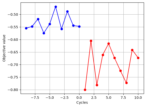
Due to the heuristic nature of the algorithms used by many Ising machines, the obtained solutions are not perfectly reproducible. Below, we show a typical example of the standard output and figure generated when running this sample code.

We were able to obtain optimization results consistent with those shown in the corresponding tutorial code.

# Objective values from the initial training data
objective_init = optimizer.training_data.y[:num_init_data]

# Objective values of the best solutions directly obtained from annealing
objective_anneal = [
    float(h.annealing_best_solution.objective) for h in optimizer.history
]

plt.plot(range(-num_init_data + 1, 1), objective_init, "-ob")
plt.plot(range(1, len(objective_anneal) + 1), objective_anneal, "-or")
plt.xlabel("Cycles")
plt.ylabel("Objective value")
plt.grid(True)
_images/4fdbe2374a72d835ae27047c8bcfb425f586ed43428acb57a2d83157934a3f00.png

Hint

In the current black-box function, the range of function values is clearly \(-1 \le y\le0\). To improve optimization performance, when applying the transformation described in this section, it is recommended to apply an offset before the exponential transformation so that the target objective value becomes zero.

\[ y^* = y + 1 \]
\[ \hat{y}=-\exp\left(\frac{-y^*}{c_m}\right) \]